ファイル:Runge phenomenon.svg
ナビゲーションに移動
検索に移動

この SVG ファイルのこの PNG プレビューのサイズ: 600 × 600 ピクセル. その他の解像度: 240 × 240 ピクセル | 480 × 480 ピクセル | 768 × 768 ピクセル | 1,024 × 1,024 ピクセル | 2,048 × 2,048 ピクセル | 720 × 720 ピクセル。
元のファイル (SVG ファイル、720 × 720 ピクセル、ファイルサイズ: 24キロバイト)
概要
| 解説 |
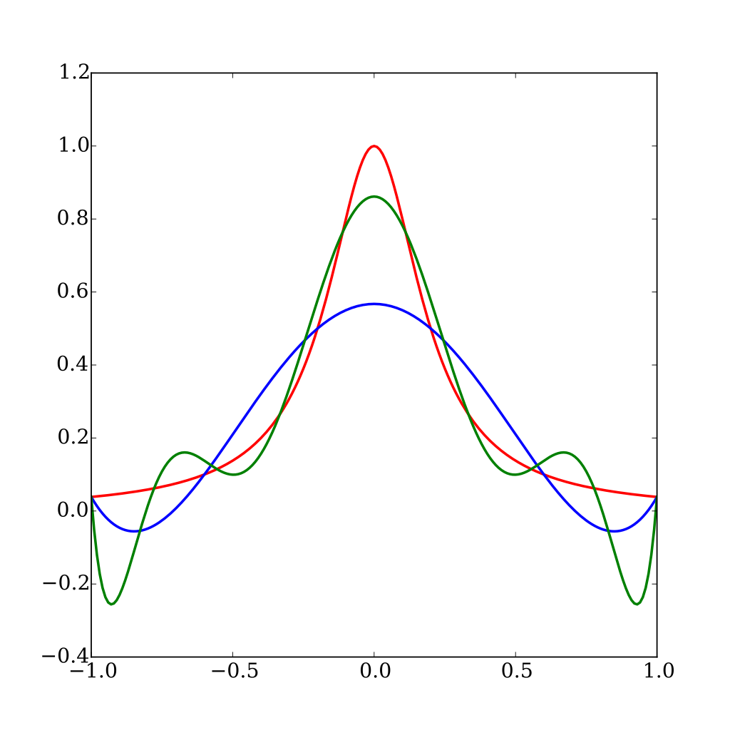
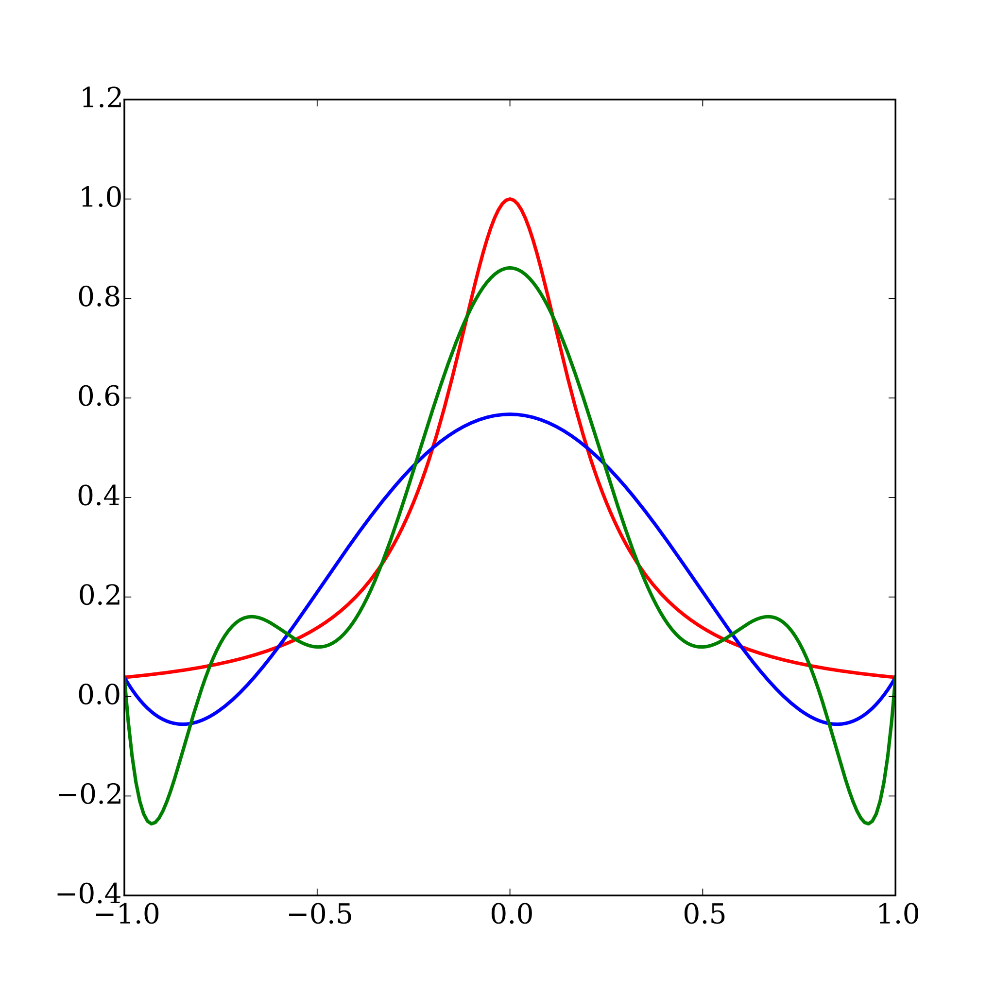
English: The red curve is the Runge function.
The blue curve is a 5th-order interpolating polynomial (using six equally spaced interpolating points). The green curve is a 9th-order interpolating polynomial (using ten equally spaced interpolating points). At the interpolating points, the error between the function and the interpolating polynomial is (by definition) zero. Between the interpolating points (especially in the region close to the endpoints 1 and −1), the error between the function and the interpolating polynomial gets worse for higher-order polynomials.Español: La curva roja es la función de Runge.
La curva azul es un polinomio interpolante de orden 5 (usando seis puntos equiespaciados). La curva verde es un polinomio interpolante de orden 9 (usando diez puntos equiespaciados). A los puntos interpolantes el error entre la función y el polinomio interpolantes es cero (por definición). Entre estos puntos (especialmente cerca de los extremos 1 y -1) el error entre la función y el polinomio interpolante incrementa conforme el polinomio aumenta de orden. |
| 日付 | |
| 原典 | 投稿者自身による著作物 |
| 作者 | Nicoguaro |
| SVG 開発 | |
| ソースコード | Python codefrom __future__ import division
import numpy as np
import matplotlib.pyplot as plt
from scipy.interpolate import lagrange
from matplotlib import rcParams
rcParams['font.family'] = 'serif'
rcParams['font.size'] = 16
def runge(x):
return 1/(1 + 25*x**2)
plt.figure(figsize=(8,8))
npts = 201
# Runge Function
x_vec = np.linspace(-1, 1, npts)
y_vec = runge(x_vec)
plt.plot(x_vec, y_vec, lw=2, color='r')
# Fifth degree polynomial
pts_x = np.linspace(-1, 1, 6)
pts_y = runge(pts_x)
poly = lagrange(pts_x, pts_y)
y_interp = poly(x_vec)
plt.plot(x_vec, y_interp, lw=2, color='b')
# Ninth degree polynomial
pts_x = np.linspace(-1, 1, 10)
pts_y = runge(pts_x)
poly = lagrange(pts_x, pts_y)
y_interp = poly(x_vec)
plt.plot(x_vec, y_interp, lw=2, color='g')
plt.savefig("Runge_phenomenon.svg")
plt.show()
|
ライセンス
この作品の著作権者である私は、この作品を以下のライセンスで提供します。
このファイルはクリエイティブ・コモンズ 表示 4.0 国際ライセンスのもとに利用を許諾されています。
- あなたは以下の条件に従う場合に限り、自由に
- 共有 – 本作品を複製、頒布、展示、実演できます。
- 再構成 – 二次的著作物を作成できます。
- あなたの従うべき条件は以下の通りです。
- 表示 – あなたは適切なクレジットを表示し、ライセンスへのリンクを提供し、変更があったらその旨を示さなければなりません。これらは合理的であればどのような方法で行っても構いませんが、許諾者があなたやあなたの利用行為を支持していると示唆するような方法は除きます。
ファイルの履歴
過去の版のファイルを表示するには、その版の日時をクリックしてください。
| 日時 | サムネイル | 寸法 | 利用者 | コメント | |
|---|---|---|---|---|---|
| 現在の版 | 2015年10月23日 (金) 00:40 | | 720 × 720 (24キロバイト) | wikimediacommons>Nicoguaro | User created page with UploadWizard |
ファイルの使用状況
以下のページがこのファイルを使用しています: